Task Scheduling Algorithms

Info

This document is a work in progress and will be updated regularly.

Introduction

Scheduling a task graph on networked computers is a fundamental problem in distributed computing. Essentially, the goal is to assign computational tasks to different compute nodes in such a way that minimizes/maximizes some performance metric (e.g., total execution time, energy consumption, throughput, etc.).

We will focus on the task scheduling problem concerning heterogeneous task graphs and compute networks with the objective of minimizing makespan (total execution time) under the related machines model¹.

It is common to model distributed applications as task graphs, where nodes represent computational tasks and directed edges represent precedence constraints and the flow of input/output data. As a result, task scheduling pops up all over the place - from machine learning and scientific workflows, to IoT/edge computing applications, to data processing pipelines used all over industry.

Figure 1 depicts a scientific workflow application used by Caltech astronomers to generate science-grade mosaics from astronomical imagery².

Figure 1a: Montage astronomical image

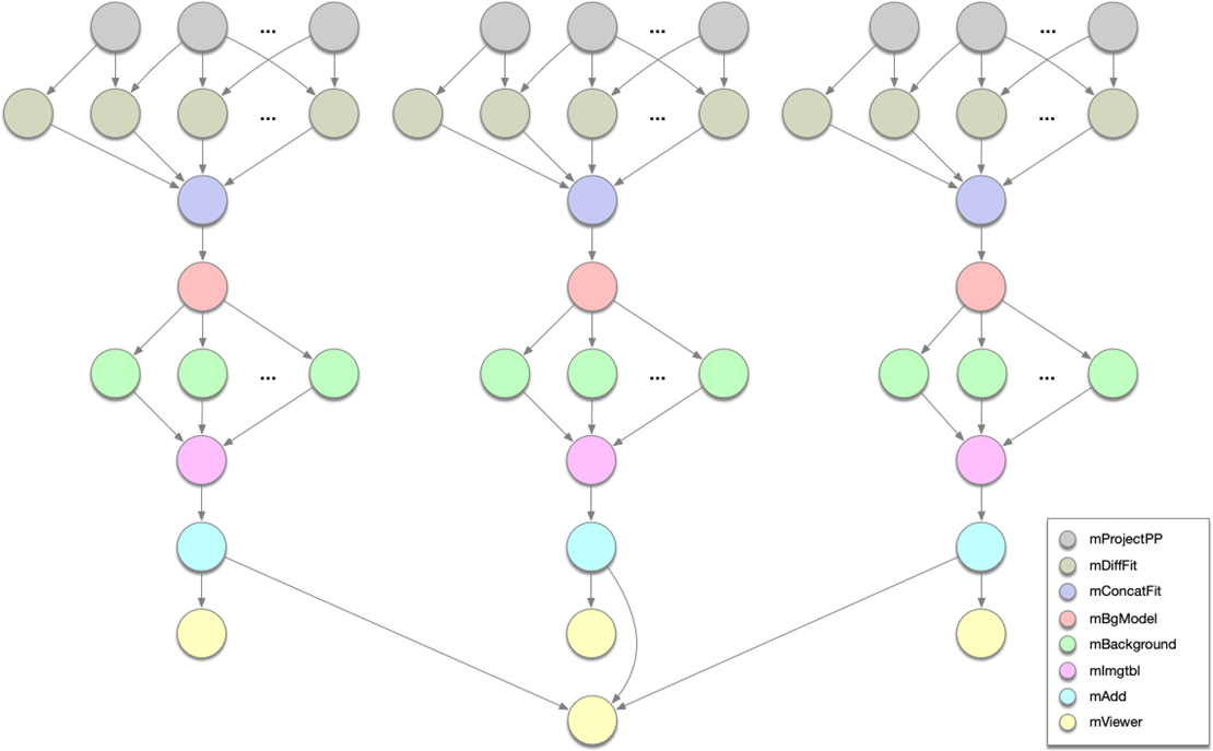Figure 1b: Montage scientific workflow structure

Problem Definition

Let us denote the task graph as $G=(T,D)$, where $T$ is the set of tasks and $D$ contains the directed edges or dependencies between these tasks. An edge $(t,t^{\prime })\in D$ implies that the output from task $t$ is required input for task $t^{\prime }$. Thus, task $t^{\prime }$ cannot start executing until it has received the output of task $t$. This is often referred to as a precedence constraint.

For a given task $t\in T$, its compute cost is represented by $c(t)\in {\mathbb{R}}^{+}$ and the size of the data exchanged between two dependent tasks, $(t,t^{\prime })\in D$, is $c(t,t^{\prime })\in {\mathbb{R}}^{+}$.

Let $N=(V,E)$ denote the compute node network, where $N$ is a complete undirected graph. $V$ is the set of nodes and $E$ is the set of edges. The compute speed of a node $v\in V$ is $s(v)\in {\mathbb{R}}^{+}$ and the communication strength between nodes $(v,v^{\prime })\in E$ is $s(v,v^{\prime })\in {\mathbb{R}}^{+}$.

Under the related machines model³, the execution time of a task $t\in T$ on a node $v\in V$ is $\frac{c(t)}{s(v)}$, and the data communication time between tasks $(t,t^{\prime })\in D$ from node $v$ to node $v^{\prime }$ (i.e., $t$ executes on $v$ and $t^{\prime }$ executes on $v^{\prime }$) is $\frac{c(t,t^{\prime })}{s(v,v^{\prime })}$.

The goal is to schedule the tasks on different compute nodes in such a way that minimizes the makespan (total execution time) of the task graph.

Let $\mathcal{A}$ denote a task scheduling algorithm. Given a problem instance $(N,G)$ which represents a network/task graph pair, let $S_{\mathcal{A},N,G}$ denote the schedule produced by $\mathcal{A}$ for $(N,G)$. A schedule is a mapping from each task to a triple $(v,r,e)$ where $v$ is the node on which the task is scheduled, $r$ is the start time, and $e$ is the end time.

A valid schedule must satisfy the following properties:

• All tasks must be scheduled: for all $t\in T$, $S_{\mathcal{A},N,G}(t)=(v,r,e)$ must exist such that $v\in V$ and $0\le r\le e$.

• All tasks must have valid start and end times: $\forall t\in T,S_{\mathcal{A},N,G}(t)=(v,r,e)⟹e-r=\frac{c(t)}{s(v)}$

• Only one task can be scheduled on a node at a time (i.e., their start/end times cannot overlap): $\forall t,t^{\prime }\in T,t\ne t^{\prime },S_{\mathcal{A},N,G}(t)=(v,r,e)\wedge S_{\mathcal{A},N,G}(t^{\prime })=(v,r^{\prime },e^{\prime })⟹e\le r^{\prime }\vee e^{\prime }\le r$

• A task cannot start executing until all of its dependencies have finished executing and their outputs have been received at the node on which the task is scheduled: $\forall (t,t^{\prime })\in D,S_{\mathcal{A},N,G}(t)=(v,r,e)\wedge S_{\mathcal{A},N,G}(t^{\prime })=(v^{\prime },r^{\prime },e^{\prime })⟹e+\frac{c(t,t^{\prime })}{s(v,v^{\prime })}\le r^{\prime }$

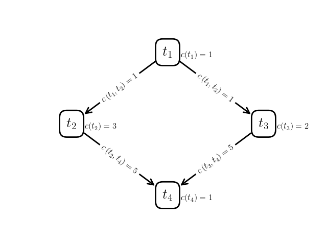Figure 2a: Example task graph

Figure 2b: Example compute network

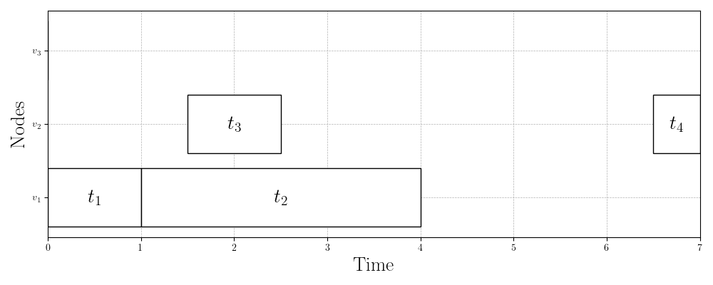Figure 2c: Example schedule (Gantt chart)

We define the makespan of the schedule $S_{\mathcal{A},N,G}$ as the time at which the last task finishes executing: $M_{\mathcal{A}(N,G)}={\max }_{t\in T\mid S_{\mathcal{A},N,G}(t)=(v,r,e)}e$

Example 1

Take a look at the task graph, network, and schedule in Figure 2. Let us start by verifying that this is a valid schedule for the problem instance (network/task graph pair).

First, task $t_1$ is scheduled to run on node $v_1$. Clearly this is valid, since $t_1$ has no dependencies. When $t_1$ finishes running at time $1$, which is valid since the cost of task $t_1$ is $1$ and the speed of node $v_1$ is $1$ ($1/1=1$).

Then, $t_2$ immediately starts running at time $1$ on node $v_1$. Again, this is clearly valid since there is no communication delay in sending the outputs from task $t_1$ to another node before running task $t_2$.

Task $t_3$, on the other hand, is scheduled to run on node $v_2$. In this case, $1$ unit of output data from task $t_1$ must be sent to node $v_2$ as input data to task $t_3$. The communication link between nodes $v_1$ and $v_2$ is $2$, so this communication takes $1/2$ units of time. Thus, the start time of task $t_3$ is valid since it is exactly $1/2$ units of time after task $t_1$ terminates.

It’s easy to verify that tasks $t_3$ and $t_2$ have valid runtimes according to their costs and the speeds of the nodes they’re running on.

Finally, task $t_4$ is scheduled to run on node $v_2$. Before it can start running, though, the $5$ units of output data from task $t_2$ must be sent from node $v_1$ to node $v_2$ over a communication link of strength $2$. Thus, the start time of task $t_4$ is correct ($5/2=2.5$ units of time after task $t_2$‘s finish time).

Thus, the schedule in Figure 2c is valid and has a makespan of $7$.

The HEFT Scheduling Algorithm

This task scheduling problem has long been known to be NP-Hard and was recently shown to also be not polynomial-time approximable within a constant factor⁴. As a result, many heuristic algorithms that aren’t guaranteed to produce an optimal schedule but that, in practice, have been shown to work reasonably well have been proposed over the past decades.

One of the most commonly used of these algorithms is HEFT (Heterogeneous Earliest Finish Time)⁵. HEFT is a list-scheduling algorithm, which essentially means it first computes priorities for each of the tasks in the task graph and then schedules the tasks greedily in order of their priority on the “best” node (the one that minimizes the task’s finish time, given previously scheduled tasks).

Here is a summary of the algorithm:

1. Calculate average compute times for each task: $\overline{\text{comp}}(t)=\frac{1}{|V|}{\sum }_{v\in V}\frac{c(t)}{s(v)}\forall t\in T$

2. Calculate average communication times for each dependency: $\overline{\text{comm}}(t_1,t_2)=\frac{1}{|E|}{\sum }_{(v_1,v_2)\in E,v_1\ne v_2}\frac{c(t_1,t_2)}{s(v_1,v_2)}\forall (t_1,t_2)\in D$

3. Calculate the upward rank of each task (recursively): $\text{urank}(t)=\overline{\text{comp}}(t)+{\max }_{t^{\prime }\in T|(t,t^{\prime })\in D}\left\{\overline{\text{comm}}(t,t^{\prime })+\text{urank}(t^{\prime })\right\}\forall t\in T$

4. In descending order of task upward ranks, greedily schedule each task on the node that minimizes its earliest possible finish time given previously scheduled tasks.

HEFT Example Calculations

Task	$\overline{\text{comp}}(t)$
$t_1$	2/3
$t_2$	2
$t_3$	4/3
$t_4$	2/3

Table 1: Average compute times for each task

$t\to t^{\prime }$	$\overline{\text{comm}}(t,t^{\prime })$
$t_1\to t_2$	2/3
$t_1\to t_3$	2/3
$t_2\to t_4$	10/3
$t_3\to t_4$	10/3

Table 2: Average communication times for each dependency

Task	$\text{urank}(t)$
$t_1$	22/3
$t_2$	6
$t_3$	16/3
$t_4$	2/3

Table 3: Upward rank of each task

Figure 3 shows three valid schedules for the same problem instance. Figure 3a shows the first schedule we validated in the previous section with makespan $7$. Figure 3b shows the schedule that the HEFT algorithm produces with a slightly better makespan of $6$. Finally, Figure 3c shows the best schedule for this problem instance, which has a makespan of just $3.5$. This is almost half the makespan of the schedule that HEFT (one of the most widely used scheduling algorithms) produces!

Figure 3a: Initial schedule (makespan = 7)

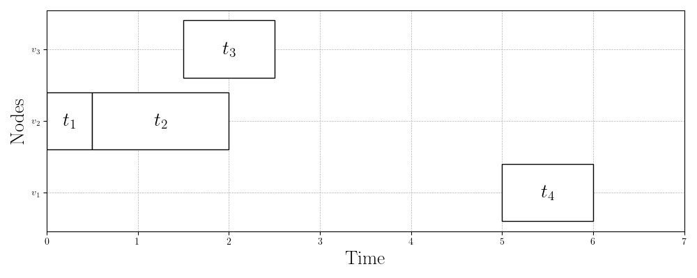Figure 3b: HEFT schedule (makespan = 6)

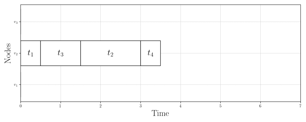Figure 3c: Optimal schedule (makespan = 3.5)

Questions to Consider

1. Upward rank has the important property that a task’s upward rank is always greater than the upward rank of its dependent tasks. Why is this important?
2. What is the runtime of HEFT in terms of $|T|$, $|D|$, $|V|$, and $|E|$?
3. Why does HEFT perform poorly on the problem instance in Figure 2? Can you think of an algorithm that would do better?

My Research Interests

Task scheduling is a fundamental problem in computer science that pops up everywhere. In this lecture, we formalized the task scheduling problem for heterogeneous task graphs and compute networks with the objective of minimizing makespan (total execution time) under the related machines model. Many other interesting variants of the task scheduling problem exist (see⁶).

We also learned HEFT, one of the most popular task scheduling heuristic algorithms, and saw a problem instance on which it performs rather poorly. Hundreds of heuristic algorithms have been proposed in the literature over the past decades (⁷ has nice descriptions of eleven scheduling algorithms). Due to their reliance on heuristics (since the problem is NP-Hard), all of these algorithms have problem instances on which they perform very poorly.

The performance boundaries between heuristic algorithms are not well-understood, however. This is an area of my research. We look at methodologies for comparing task scheduling algorithms to better understand the conditions under which they perform well and poorly.

Figures 4 and 5 depict results from our efforts in this area. Figure 4 shows benchmarking results for 15 scheduling algorithms on 16 datasets. The color represents the maximum makespan ratio (MMR) of an algorithm on a problem instance in a given dataset. The MMR of an algorithm is essentially how many times worse the algorithm performs on a particular problem instance compared to the other scheduling algorithms. For example, on some problem instances in the cycles dataset, the BIL algorithm performs more than five times worse than another one of the 15 algorithms! On other problem instances in the same dataset, however, the algorithm performs well (MMR=1).

Figure 5 shows results from our own comparison method that pits algorithms against each other and tries to find a problem instance where one algorithm maximally underperforms compared to another. Our hope is that by identifying these kinds of problem instances, we can better understand the conditions under which algorithms perform well/poorly.

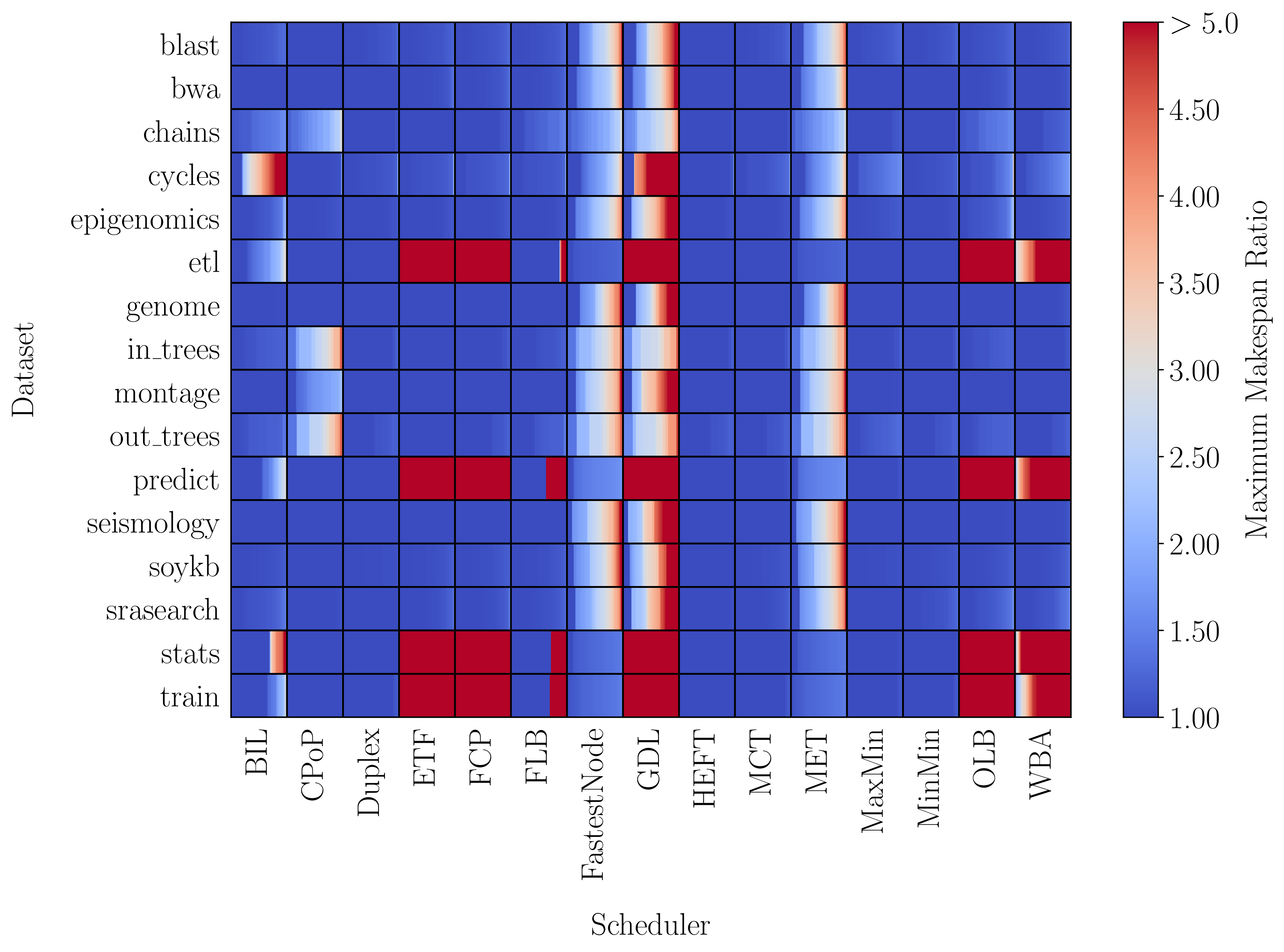Figure 4: Benchmarking results for 15 scheduling algorithms on 16 datasets

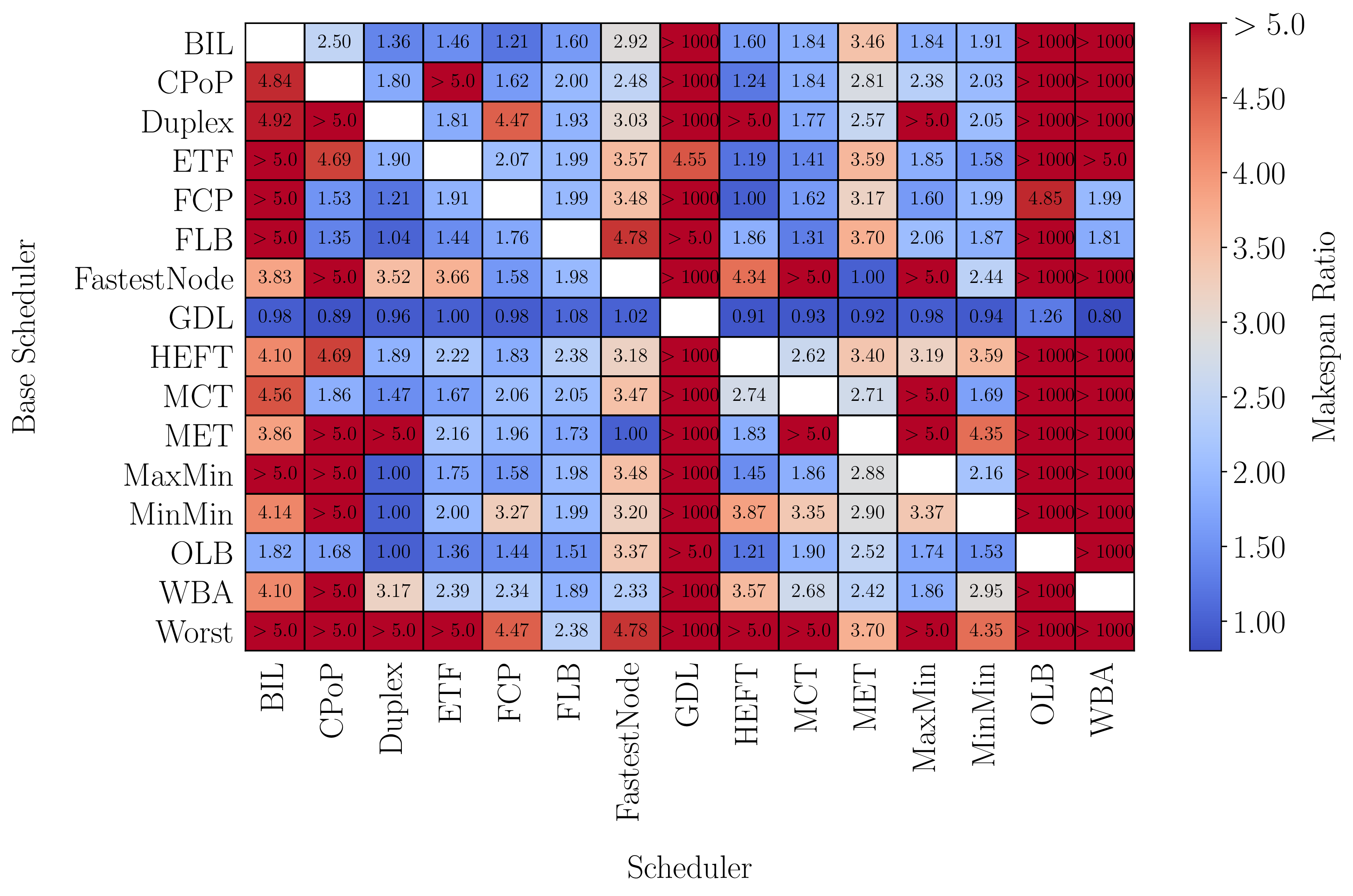Figure 5: Adversarial analysis results for 15 scheduling algorithms

Theory

Scheduling Algorithms

Surveys and Algorithm Comparison Papers

Machine Learning Approaches

Data and Other References

Footnotes

1. In the related machines model, if the same task executes faster on some compute node $n_1$ than on node $n_2$, then $n_1$ must execute all tasks faster than $n_2$ ($n_1$ is strictly faster than $n_2$). Note that this model cannot describe multi-modal distributed systems, where certain classes of tasks (e.g., GPU-heavy tasks) might run better/worse on different types of machines (e.g., those with or without GPUs). ↩

2. M. Rynge et al. 2014. “Producing an Infrared Multiwavelength Galactic Plane Atlas Using Montage, Pegasus, and Amazon Web Services.” In Astronomical Data Analysis Software and Systems XXIII, 211. ↩

3. R. L. Graham. 1969. “Bounds on Multiprocessing Timing Anomalies.” SIAM Journal on Applied Mathematics 17(2): 416-429. DOI: 10.1137/0117039 ↩

4. Abbas Bazzi and Ashkan Norouzi-Fard. 2015. “Towards Tight Lower Bounds for Scheduling Problems.” In Algorithms - ESA 2015, 118-129. DOI: 10.1007/978-3-662-48350-3_11 ↩

5. Haluk Topcuoglu, Salim Hariri, and Min-You Wu. 1999. “Task Scheduling Algorithms for Heterogeneous Processors.” In 8th Heterogeneous Computing Workshop, 3-14. DOI: 10.1109/HCW.1999.765092 ↩

6. R.L. Graham, E.L. Lawler, J.K. Lenstra, and A.H.G. Rinnooy Kan. 1979. “Optimization and Approximation in Deterministic Sequencing and Scheduling: a Survey.” In Discrete Optimization II, Annals of Discrete Mathematics 5: 287-326. DOI: 10.1016/S0167-5060(08)70356-X ↩

7. Tracy D. Braun et al. 2001. “A Comparison of Eleven Static Heuristics for Mapping a Class of Independent Tasks onto Heterogeneous Distributed Computing Systems.” Journal of Parallel and Distributed Computing 61(6): 810-837. DOI: 10.1006/jpdc.2000.1714 ↩